From Gated DeltaNet to Kaczmarz
Many linear attention variants can be viewed as maintaining a matrix $S_t$ that linearly maps keys to values. Gated DeltaNet [1] is special in that it does not write $K_t^\top V_t$ directly, but instead writes the prediction residual, and uses gating to control forgetting and write strength.
1. Update formula of Gated DeltaNet
At time $t$, we are given $K_t \in \mathbb{R}^{1\times d_k}$ and $V_t \in \mathbb{R}^{1\times d_v}$ as row vectors, together with the memory matrix $S_t \in \mathbb{R}^{d_k\times d_v}$.
The core recurrence of Gated DeltaNet is:
\[\begin{aligned} e_t &= V_t - K_t S_{t-1} \\ S_t &= \alpha_t S_{t-1} + \beta_t K_t^\top e_t \end{aligned}\]The gating is usually produced from the input $X$:
- $\beta_t = \sigma(\mathrm{Linear}_\beta(X))$ represents the write strength.
- $\alpha_t \in (0,1]$ is the forgetting/decay coefficient, controlling what fraction of the old memory $S_{t-1}$ is retained.
2. Online learning perspective
We can view $S$ as the weights of a multi-output linear regression: $\hat V_t = K_t S$. The single-sample online ridge regression loss is:
\[\ell_t(S)=\frac12\|V_t-K_tS\|_F^2+\frac{\lambda_t}{2}\|S\|_F^2\]Its gradient is:
\[\nabla_S\ell_t(S)=-K_t^\top e_t+\lambda_t S\]If we take one step of gradient descent (with learning rate $\beta_t$):
\[\begin{aligned} S_t &=S_{t-1}-\beta_t\nabla_S\ell_t(S_{t-1})\\ &=(1-\beta_t\lambda_t)S_{t-1}+\beta_tK_t^\top(V_t-K_tS_{t-1}) \end{aligned}\]Comparing with the form of Gated DeltaNet:
\[S_t=\alpha_tS_{t-1}+\beta_tK_t^\top(V_t-K_tS_{t-1})\]We obtain the exact correspondence: $\alpha_t = 1-\beta_t\lambda_t$. In practice, implementations often use $\alpha_t=\exp(g_t)$ for numerical stability.
3. Introducing the Kaczmarz algorithm
From the constraint perspective, SGD is not the only optimization method. Once we put more weight on the geometry of constraint satisfaction, each token can be viewed as a linear constraint $K_tS = V_t$.
One step of Kaczmarz can be defined as follows: among the set of $S$ satisfying the current constraint, find the one closest to the previous solution, i.e., the minimal-change projection:
\[S_t=\arg\min_S\frac12\|S-S_{t-1}\|_F^2\quad\text{s.t.}\quad K_tS=V_t\]We can solve this using the Lagrange multiplier method. Construct the Lagrangian:
\[\mathcal{L}(S,\lambda)=\frac12\|S-S_{t-1}\|_F^2+\lambda(K_tS-V_t)\]Take the derivative with respect to $S$ and set it to zero:
\[\nabla_S\mathcal{L}=(S-S_{t-1})+K_t^\top\lambda=0 \Rightarrow S=S_{t-1}-K_t^\top\lambda\]Substitute $S$ back into the constraint $K_tS=V_t$:
\[K_t(S_{t-1}-K_t^\top\lambda)=V_t \Rightarrow K_tS_{t-1}-\|K_t\|_2^2\lambda=V_t\]Solving gives:
\[\lambda=-\frac{V_t-K_tS_{t-1}}{\|K_t\|_2^2} = -\frac{e_t}{\|K_t\|_2^2}\]Thus we obtain the Kaczmarz recurrence:
\[\boxed{ S_t=S_{t-1}+\frac{1}{\|K_t\|_2^2}\,K_t^\top e_t }\]4. Geometric interpretation
The Kaczmarz algorithm has a clear geometric interpretation:
- Projection interpretation: The Kaczmarz update step projects $S_{t-1}$ onto the hyperplane ${S:K_tS=V_t}$.
- Error elimination: When using hard projection, the updated $S_t$ satisfies the current constraint, i.e., $K_tS_t=V_t$.
- Optimal step size: It can be viewed as a single gradient step with the optimal step size. If we perform an exact line search along the gradient direction for the instantaneous squared error, the optimal step size is $1/|K_t|^2$.
- QK Norm perspective: This normalization factor also explains QK Norm, a trick added at the implementation level in today’s Attention / Linear Attention; here we introduce it explicitly.
5. Generalization to inconsistent constraints
In practice, constraints are often inconsistent or noisy, and no single $S$ can satisfy all of them simultaneously. Hard projection may make the model oscillate or overfit the current sample.
Therefore, Relaxed Kaczmarz (or Damped Kaczmarz) is commonly used, introducing a relaxation coefficient $\rho_t$ in the numerator and adding a numerical stability term $\varepsilon$ in the denominator:
\[\boxed{ S_t = S_{t-1} + \frac{\rho_t}{\|K_t\|_2^2+\varepsilon}\,K_t^\top\bigl(V_t-K_tS_{t-1}\bigr) }\]This update formula satisfies the following property:
\[K_tS_t=(1-\rho_t)K_tS_{t-1}+\rho_tV_t\]That is, the new prediction is a linear interpolation between the old prediction and the target value.
Combined with the forgetting mechanism of Gated DeltaNet, this gives an update that first forgets and then projects:
\[\tilde S_{t-1}=\alpha_tS_{t-1},\qquad S_t=\tilde S_{t-1}+\frac{\rho_t}{\|K_t\|^2+\varepsilon}K_t^\top\bigl(V_t-K_t\tilde S_{t-1}\bigr)\]6. Connection with Longhorn
Longhorn [2] adopts a smoother update strategy, replacing the hard constraint projection with a proximal objective:
\[S_t=\arg\min_S\frac12\|S-S_{t-1}\|_F^2+\frac{\gamma_t}{2}\|V_t-K_tS\|_F^2\]Its closed-form solution is:
\[\boxed{ S_t = S_{t-1} + \frac{\gamma_t}{1+\gamma_t\|K_t\|_2^2} K_t^\top\bigl(V_t-K_tS_{t-1}\bigr) }\]This coefficient can be rewritten as:
\[\frac{\gamma_t}{1+\gamma_t\|K_t\|^2} = \frac{1}{\|K_t\|^2+\frac{1}{\gamma_t}}\]Setting $\varepsilon_t = 1/\gamma_t$ then shows that Longhorn is similar to Kaczmarz.
7. Method comparison table
| Method | State Update | Effective Step Size |
|---|---|---|
| Gated DeltaNet | $S_t=\alpha_tS_{t-1}+\beta_tK_t^\top e_t$ | $\beta_t$ |
| Kaczmarz | $S_t=S_{t-1}+\frac{1}{|K_t|^2}K_t^\top e_t$ | $\frac{1}{|K_t|^2}$ |
| Relaxed Kaczmarz | $S_t=S_{t-1}+\frac{\rho_t}{|K_t|^2+\varepsilon}K_t^\top e_t$ | $\frac{\rho_t}{|K_t|^2+\varepsilon}$ |
| Longhorn / Prox | $S_t=S_{t-1}+\frac{\gamma_t}{1+\gamma_t|K_t|^2}K_t^\top e_t$ | $\frac{1}{|K_t|^2+1/\gamma_t}$ |
8. Experiments
We trained on the SlimPajama dataset for 100 million tokens and plotted validation perplexity (ppl) and loss as a function of token horizon. In the figure, @1x and @2x correspond to evaluation results with sequence lengths 2048 and 4096, respectively.
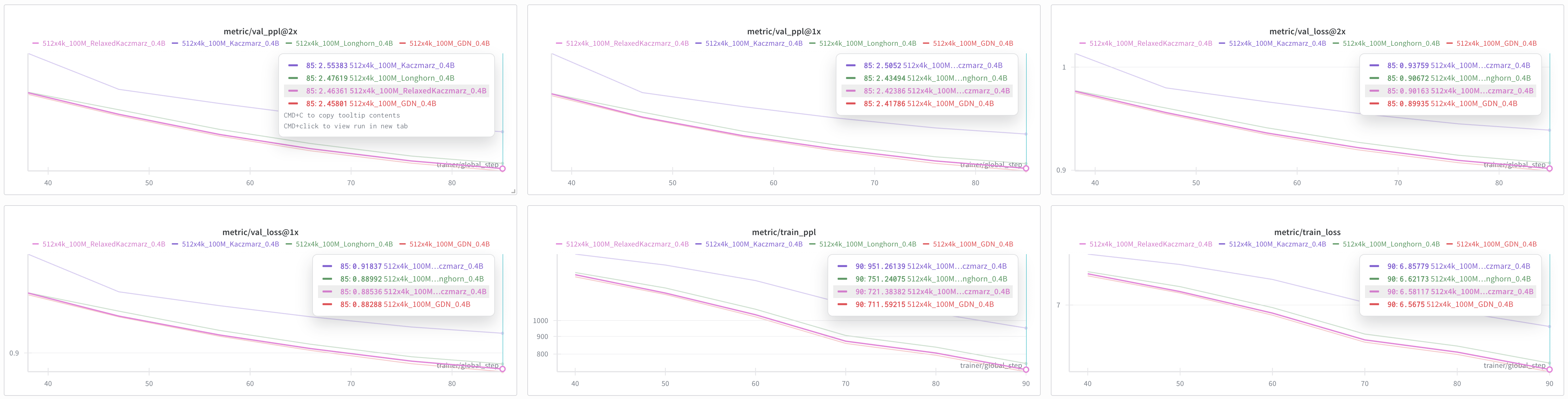
If Longhorn can be viewed as a form of Kaczmarz, then Relaxed Kaczmarz should be better, which the experiments confirm. Gated DeltaNet also uses the QK Norm trick; once we add the Q Norm trick as well, Relaxed Kaczmarz + Q Norm becomes comparable to Gated DeltaNet.
References
[1] Yang, S., Kautz, J., & Hatamizadeh, A. (2025). Gated Delta Networks: Improving Mamba2 with Delta Rule. arXiv preprint arXiv:2412.06464.
[2] Liu, B., Wang, R., Wu, L., Feng, Y., Stone, P., & Liu, Q. (2024). Longhorn: State Space Models are Amortized Online Learners. arXiv preprint arXiv:2407.14207.
Citation
If you need to cite this article, please refer to:
@article{zou2026kaczmarz,
  title={从 Gated DeltaNet 到 Kaczmarz},
  author={Zou, Jiaxuan},
  journal={Jiaxuan's Blog},
  year={2026},
  url={https://jiaxuanzou0714.github.io/blog/2026/kaczmarz/}
}