How to Build a Scientific Scaling Ladder
This article draws on publicly available literature and engineering practice, and contains no proprietary information. It covers how to build a scientific Scaling Ladder—fitting Scaling Laws on small-model experiments and extrapolating large-model configurations and performance.
1. Core Concepts and Objectives
1.1 What Is a Scaling Ladder
A Scaling Ladder is a set of experiment points spanning different parameter counts $N$ and training data sizes $D$, used to fit Scaling Laws and extrapolate large-model performance. The layout of experiment points and each point’s role in fitting versus validation are detailed in §4.1.
1.2 Why a Scientific Ladder Is Needed
Scaling Laws fit empirical regularities on small models and extrapolate to predict the training configuration, loss, and downstream performance of large models, providing quantitative guidance for choosing model size, training budget, and hyperparameters and reducing configuration risk in large-scale training.
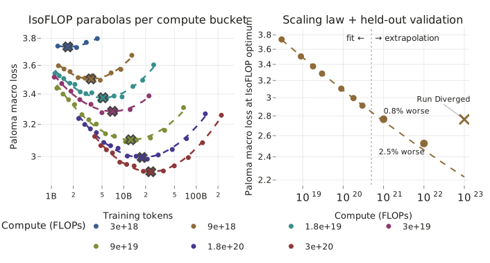
A scientific Scaling Ladder should be validated for extrapolation accuracy on the delivered model. The acceptance threshold depends on the minimum distinguishable difference between target configurations and random-seed variance (see §7.1); a relative error of ≤ 0.02 on Training Loss can serve as a reference.
1.3 Core Outputs of a Ladder
The outputs of a Scaling Ladder include:
| Output | Prediction Target |
|---|---|
| Hyperparameter Scaling Law (LR/BSZ/WD) | Optimal training hyperparameters |
| Loss Scaling Law | Final Training/Eval Loss |
| Loss Curve Scaling Law | Full training curve |
| Annealing ratio Scaling Law | Optimal LR decay ratio |
| Data repetition Scaling Law | Effective performance under multi-epoch training |
| Downstream task Scaling Law | Benchmark metrics |
| … | … |
1.4 Decision Objectives
A Scaling Ladder supports four types of decisions:
- Fixed-recipe prediction: predicting a given recipe’s performance at target scale. An effective scaling law does not require exhaustive tuning at every experiment point.
- Optimal resource allocation: choosing the allocation of parameters $N$ and training budget $D$ under a compute constraint.
- Candidate comparison: comparing different architectures, optimizers, or data recipes.
- Hyperparameter prediction: predicting hyperparameters across scales or training budgets.
Before building, one should determine the objective type and specify the target model, training stage, budget constraint, inference deployment conditions, and which prediction errors would change the final decision. Delphi (Marin, 2026) examines competitiveness and predictability separately; both require independent validation. The Fully-Tuned Frontier requirement of §5.1 applies to objectives 2 and 3; objective 1 only needs fitting along the recipe.
2. Evaluation Protocol and Acceptance Criteria
Before building a Ladder, the evaluation protocol must be defined:
- Proxy versus final metrics: proxy metrics (training loss, answer BPB) and final acceptance metrics (downstream benchmark accuracy) should be specified separately. Loss improvements at small scale do not guarantee downstream improvements at target scale (Qwen3.8-Next, 2026 §1).
- Signal distinguishability: each metric must carry a distinguishable signal at the Ladder’s fitting scales. Small models may perform near random on math or code tasks, and some metrics saturate at large scale—neither case supports decisions. For tasks where accuracy cannot discriminate, use continuous proxy metrics such as answer BPB (OLMo 3, 2025).
- Cross-scale rank correlation: when proxy metrics are used for candidate selection, rank correlation with target-scale capability metrics must be established (OLMo 3, 2025 §3.3, Appendix A.4).
- Evaluation version control: record prompt templates, generation settings, scoring methods, and versions; check for train–evaluation data overlap.
- Coverage of target capabilities: specify which delivery capabilities the evaluation tasks cover, how they are aggregated, and the tolerance for critical single-task degradation. High-noise tasks may require increased sampling or separate reporting (Phi-4, 2024 §5; OLMo 3, 2025 §3.3.3–3.3.4).
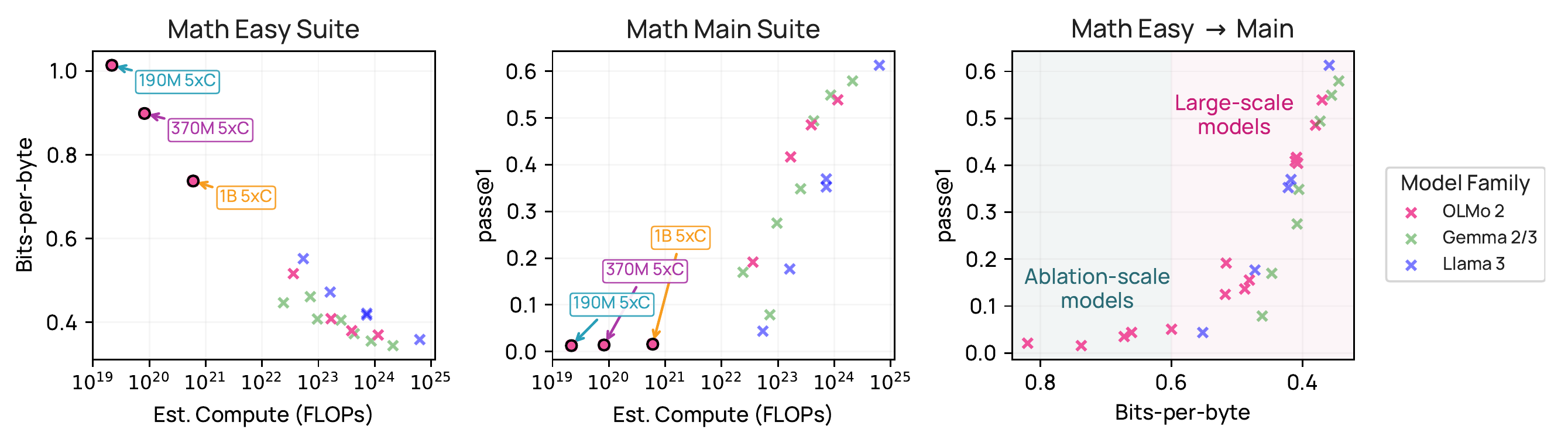
When transfer evidence for proxy conclusions is insufficient, the applicable scope and items awaiting validation should be stated.
If the delivered model undergoes post-training (SFT/RL), representative candidates should be validated through comparably conditioned post-training. Qwen3.8-Next, 2026 reports two modifications each with small pre-training impact: NoPE led to non-terminating generation after post-training, and the sparse read-residual branch led to quality degradation after post-training. OLMo 3, 2025 §3.5.1 conducts rapid instruction tuning on candidates after full annealing. Post-training acceptance should check termination behavior, output length, and other delivery metrics beyond capability scores.
3. Baseline Recipe and Model Sizing
3.1 Parameter Count Convention
The parameter count conventions for fitting $L(N,D)$ and computing $C$ differ and must be recorded separately.
This article uses the Transformer body parameter count $N_{\text{body}}$ for fitting $L(N,D)$, excluding the input embedding and output head. Embedding/head scales as $O(Vd)$ while the body scales as $O(d^2 n)$, and the ratio between the two varies with model size. Farseer (Li et al., 2025) Appendix G ablations show that including embeddings increases extrapolation error at 25.1B; Kaplan et al., 2020 also excludes embeddings. When citing other work, note their parameter count definition.
When computing $C$, the output head must be included (one $d \times V$ matmul per token), so substituting $N_{\text{body}}$ directly into $6ND$ underestimates this cost. One can approximate parameter-related matmul cost as $6(N_{\text{body}}+Vd)D$, then add attention computation.
The input embedding is a table lookup by token ID; this article records its parameters and memory access cost separately. Weight tying reduces storage, but the output head computation must still be counted. External conventions differ: Porian’s $N$ includes the output head but excludes the input embedding (Porian et al., 2024 Table 2); Chinchilla’s 20 TPP is based on total parameters including embeddings.
3.2 Compute and Width-Depth Ratio
The common approximation $C\approx6ND$ omits attention matrix operations. For standard MHA, $4d$ FFN, and full attention:
\[C \approx \left(6 + \frac{L}{d}\right) N_{\text{body}}D + 6VdD\]$L$ is the sequence length, $d$ the hidden dimension, $V$ the vocabulary size. The $L/d$ term comes from attention; the trailing term is the output head. SwiGLU, GQA, MoE, etc. change the coefficients; compute should be tallied per actual architecture.
Under the above architecture, $N_{\text{body}}\approx12d^2n$ ($n$ = number of layers). For a given parameter count, width-depth configurations still affect actual compute; the Ladder should record the structural scaling rule and use actual $C$.
Kaplan et al., 2020 reported that for a given parameter count the width-depth ratio had little effect on loss over a wide range, but subsequent experiments showed differences on benchmarks (Gemstones, 2025 §4.4) and reasoning capability (GLM-4.5, 2025). Within a Ladder, a consistent width-depth scaling rule should be used; add representative controls when structural choices are under study.
3.3 Architecture Consistency
Within one model family, except for architecture variables under explicit study, each experiment point should maintain consistent attributes or scaling rules:
| Attribute | Requirement |
|---|---|
| Architecture type | Consistent, e.g., all decoder-only Transformer |
| Normalization | Consistent, e.g., all RMSNorm |
| Positional encoding | Consistent, e.g., all RoPE |
| Activation function | Consistent, e.g., all SwiGLU |
| Embedding sharing | tied / untied consistent within the Ladder |
| Attention type | Consistent, e.g., all GQA |
| Width-depth configuration | Scaled by a predefined rule; add representative controls when structural choices are under study (§3.2) |
3.4 Shared Configuration and Variable Classification
Within one recipe, except for variables under explicit study, the following training configurations should be kept consistent (architecture rules in §3.3):
| Configuration | Example |
|---|---|
| Sequence length | 4,096 |
| Training data version | Same version |
| Optimizer | AdamW |
| Evaluation set | Same eval set |
| Evaluation frequency | Set as a fixed fraction of training progress |
Evaluation frequency note: a fixed step interval causes different effective eval point counts across different training lengths. Setting it as a fixed fraction of total steps $T$ makes the eval point count approximately equal across configurations.
Variables in the Ladder should be classified:
| Variable Category | Meaning | Examples |
|---|---|---|
| Fixed | Same value across all Ladder points | Architecture, data version, optimizer type, seq_len |
| Scaling rule | Changes with $N$ or $D$ by a predefined rule | LR (power law or $\mu$P), BSZ ($D^{0.4}$ as a prior to be validated), warmup |
| Experimental independent variable | Quantity to be fitted or searched | $N$, $D$, final optimal LR and BSZ |
After changes to architecture, optimizer, data, or precision, first verify transferability at small scale before deciding on local recalibration or full refitting. Tokenizer, initialization, parameterization, and loss accounting conventions should also be kept consistent within the Ladder.
4. Experiment Matrix and Training Budget Design
4.1 Experiment Matrix Structure
Training budget D →  0.5×    1×     2×     4×
Model   130M          ●      ●      ●      ●
size    520M          ●      ●      ●      ●
        2.3B          ●      ●      ●      ●
N       8B            ○      ○      ○      ○  ← holdout (excluded from fitting)
↓
Design principles:
- Fitting points: smaller sizes used for fitting Scaling Laws
- Holdout points: the largest size is excluded from fitting to validate extrapolation accuracy
- Specific recommendations for size and training-budget tiers are in §4.2
The sizes, training budgets, and full-grid layout above are illustrative; actual layouts should be chosen based on decision objectives, functional form, and budget.
The experiment point layout and functional form should be designed jointly. When designing the matrix, specify the fitting and target ranges for $N$, $D$, and data repetition degree, distinguishing extrapolation along $N$, along $D$, and joint extrapolation. Based on the objective from §1.4, choose a full grid, IsoFLOP, or sparse layout (see §6.1). Reserve validation points in advance, and specify what results trigger supplementary experiments. Search, seed, evaluation, validation, and supplementary experiments should all count toward the total budget.
4.2 Number of Sizes and Range
The number of sizes and range should be determined jointly with the functional form, extrapolation target, and budget:
| Dimension | Recommendation | Source |
|---|---|---|
| Number of model sizes | Cover the target extrapolation direction, plus a separate holdout; adding sizes checks fitting stability | Choshen et al., 2025 |
| Size range | Cover the target extrapolation interval; 34× is still usable on some families | Choshen et al., 2025 |
| Adjacent size ratio | Can use geometric progression; specific spacing depends on budget | Design recommendation |
| Number of training-budget tiers | Cover different training lengths per objective; Fantastic Optimizers uses 4 tiers | Fantastic Optimizers (Wen et al., 2025) |
| Training-budget range | Fantastic Optimizers uses 1×, 2×, 4×, 8× Chinchilla ratio | Fantastic Optimizers (Wen et al., 2025) |
Intermediate checkpoints can be included in fitting, but their early-training impact must be checked. Choshen et al., 2025 found that excluding early checkpoints reduces prediction error; their cutoff at the first 10% or first 10B tokens should not be applied directly to all training budgets. The cutoff rule should be determined in advance, or model sizes should be split into fitting, validation, and test segments (Lourie et al., 2026). Random-seed variance should also be incorporated into the experimental design.
4.3 Published Scale Configurations
Published model-scale and training-budget configurations for reference:
| Source | Model Parameters (per each source’s convention) | Training Budget | Reference |
|---|---|---|---|
| OpenAI | Multiple sizes, largest 1.5B (non-embedding params) | 22M–23B tokens | Kaplan et al., 2020 |
| DeepMind Chinchilla | 70M–16B (400+ models) | 5B–500B tokens | Hoffmann et al., 2022 |
| StepFun | Multiple sizes (3,700+ models) | Cumulative 100T tokens across all experiments | Step Law (Li et al., 2025) |
| Gadre et al. | 11M–6.9B (104 models) | Up to 32× Chinchilla ratio | Gadre et al., 2024 |
| Fantastic Optimizers | 0.1B–1.2B (4 sizes) | 1×–8× Chinchilla ratio | Wen et al., 2025 |
| Delphi | Sizes and budgets swept per compute budget, largest holdout 25B | Fitting 3e18–3e20 FLOPs, holdout up to 1e23 FLOPs | Marin, 2026 |
| NVIDIA Nemotron | 15B, 340B | 8T, 9T tokens | 15B report; 340B report |
| OLMo | 1B, 7B, 13B, 32B (released models) | OLMo 1: 2T–2.46T; OLMo 2: multi-stage budgets per model | OLMo, 2024; OLMo 2, 2025 |
4.4 Compute-Optimal Ratio
Chinchilla’s (Hoffmann et al., 2022) IsoFLOP method: fix each compute budget $C$, train models of different sizes, and take the minimum of the loss curve to obtain the optimal $(N, D)$ combination at that budget.
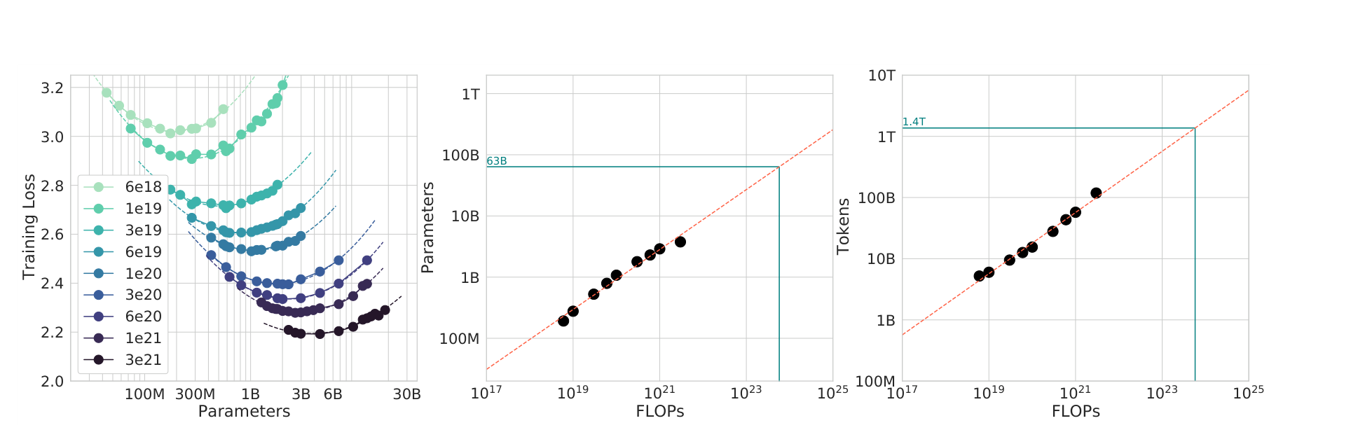
From 400+ models (70M–16B, 5B–500B tokens):
\[N_{opt}\propto C^a,\qquad D_{opt}\propto C^b,\qquad a\approx b\approx0.5\]That is, within this range, model and data scale approximately proportionally; exact exponents vary slightly across fitting methods. The parameterized loss takes the form $L(N,D)=E+A/N^\alpha+B/D^\beta$.
Gadre et al., 2024 found across 104 models that the power-law exponent of Loss vs. $C$ is similar under different $D/N$ ratios, providing empirical evidence for extrapolation in the over-training regime (up to 32× Chinchilla).
4.5 Ladder Training-Budget Tiers
Start the design from 0.5×–4× Chinchilla ratio, covering under-trained to over-trained; these tiers are illustrative—the actual range should cover the target training budget. Chinchilla’s $D/N\approx20$ tokens/parameter is based on total parameters including embeddings (Appendix F); the ratio is larger when converted to $N_{\text{body}}$, and the optimal ratio must be validated on one’s own recipe.
4.6 Impact of Data Quality on Scaling Laws
DeepSeek LLM, 2024 observed across the training corpora compared:
- Higher-quality corpora correspond to optimal compute allocations more skewed toward parameter count
- Scaling law parameters differ significantly across datasets and cannot be directly reused
- Under controlled recipe and evaluation distribution, differences in optimal $N/D$ can help judge data quality
After data version changes, scaling law parameters must be re-validated. Evaluating new data sources does not require rerunning the full matrix: OLMo 2, 2025’s Micro-annealing starts from a designated checkpoint, mixes candidate data with general data for short-term annealing, and can determine the gain. The conclusions of this method are limited to the starting checkpoint and stage, and cannot infer full-training data rankings.
4.7 Data-Mix Ladder
A Data-Mix Ladder fixes model architecture, parameter count, training budget, and optimizer, varying only the data mixing vector $\mathbf{w}=(w_1,\ldots,w_k)$.
OLMo 3, 2025 samples candidate mixes from a Dirichlet distribution, trains a 30M proxy model on each (3B tokens, ~5× Chinchilla), fits a model from mix to task performance using answer BPB, and solves for the optimal mix under token budget and repetition constraints. Inter-domain proportion and intra-domain quality distribution are optimized separately. Qwen3, 2025 extends the mix axis to instance attributes (educational value, domain, language, safety).
Mix experiments select the training distribution; scale Ladders fit $N$, $D$, and loss on that distribution. If the mix is adjusted with training budget, the two types of experiments must iterate. Proxy experiments can simultaneously scale down training budget and per-bucket data pools to preserve repetition counts (Marin data pipeline, 2026 §3; transfer to larger models remains to be validated). Data selection for training from scratch versus continued training should be handled separately, each with its stated transfer scope.
4.8 Data Repetition Scaling Law
Multi-epoch training requires distinguishing cumulative training tokens, unique tokens, and repetition count.
Muennighoff et al., 2023 assumes exponentially decaying marginal returns, yielding an equivalent data quantity:
\[D^{\prime} = U_D + U_D \cdot R_D^{\ast} \left(1 - e^{-R_D / R_D^{\ast}}\right)\]$U_D$ is the number of unique tokens, $R_D$ is the additional repetition count ($R_D=0$ means single epoch), $R_D^\ast$ is the fitted decay scale. As $R_D\to\infty$, $D^\prime\to U_D(1+R_D^\ast)$. This form describes return saturation; if loss increases with further repetition, an overfitting term must also be modeled.
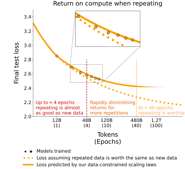
Guidance for Ladder design:
- The upper bound on repetition depends on data and recipe. Yan et al., 2025 derives under linear-regression assumptions that the optimal repetition count grows logarithmically with sample size; Lovelace et al., 2026 finds that larger parameter counts, fewer unique tokens, and more repetitions jointly exacerbate overfitting.
- In the controlled experiments of Xue et al., 2023, repetition overfitting varies primarily with parameter count; increasing data quantity mitigates it, but improving quality at the same data quantity does not yield the same improvement. Dropout noticeably alleviates repetition overfitting (v2 Table 4); the rate needs re-tuning for larger models.
5. Hyperparameter Search and Training Execution
This chapter calibrates fully-tuned $(\eta,B)$ and writes them as functions that can extrapolate with $N,D$ (or $C$); fixed-recipe prediction (§1.4 objective 1) runs according to the recipe’s scaling rule.
5.1 Search Objective: Fully-Tuned Frontier and Wide Plateau
Lourie et al., 2026 and Step Law (Li et al., 2025) reveal: small models degrade steeply under sub-optimal hyperparameters, and the Scaling Law only manifests on the Fully-Tuned Frontier; insufficient search distorts the power-law curve, leading to inaccurate large-model predictions.
Large-model experiments, however, observe a wide near-optimal region. Qwen3.8-Next, 2026 tested LR $\times/\div\,\sqrt{2}$ and BSZ +25% on a 156B-A7B model; the final training loss differed by at most $7\times10^{-4}$.
Resource allocation principle for search (§1.4 objectives 2–4): concentrate compute on exhaustive search at small scales to ensure fitting points lie on the Fully-Tuned Frontier; at large scale, first confirm locally within the extrapolated LR $\times/\div\,\sqrt{2}$ range, expanding the search if necessary. Objective 1 runs according to the recipe’s scaling rule.
5.2 Weight Decay Handling
Several published recipes fix WD (Kimi K2, 2025 $\lambda=0.1$; OLMo 3, 2025 AdamW, embeddings excluded from decay; Qwen3, 2025 does not report WD scaling). The optimal WD depends on training budget and evaluation objective: Han et al., 2026 found that the WD preferred by pre-training loss decreases with higher TPP, while stronger WD may benefit post-training plasticity. When replicating a recipe, follow its WD; when studying full tuning or cross-TPP relationships, check WD impact. Under AdamW, the Power Lines (Bergsma et al., 2025) timescale $\tau=B/(\eta\lambda D)$ can be used for joint calibration.
5.3 Batch Size and Learning Rate Transfer Rules
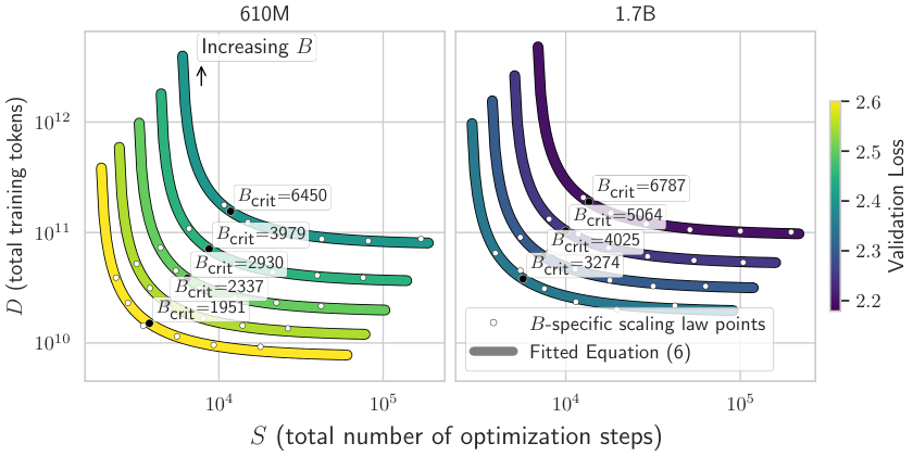
Power Lines (Bergsma et al., 2025) measured: \(B_{opt}\propto D^{0.4},\qquad B_{crit}\propto D_{min}^{0.5}\) $D$ is the training budget, $D_{min}$ is the minimum tokens needed to reach a target loss. The above exponents are approximate fitting results from that work, and $B_{opt}$ and $B_{crit}$ depend weakly on $N$. Use these to initialize BSZ transfer rules, validating on your own data.
$B_{crit}$ is the trade-off knee between token efficiency and step count: in that work’s hyperbolic model, at $B=B_{crit}$ reaching the same loss requires approximately $2D_{min}$ tokens; further increasing $B$ reduces steps but increases token and compute cost. Actual training time also depends on hardware utilization and requires system-level benchmarking.
Schaipp, 2026 defines a near-optimal batch interval at ~5% compute loss; the measured width is approximately 4×; under that work’s log-symmetric fitting model this corresponds to $[B_{opt}/2,2B_{opt}]$, which can serve as a starting point for local search.
When $B < B_{crit}$, Power Lines adjusts $\lambda$ to maintain the optimal timescale $\tau = B/(\eta\lambda D)$; LR is further constrained by the maximum stable learning rate (Power Lines §2.4). When extrapolating $B_{opt}\propto D^{0.4}$ to different training budgets, $\lambda$ and $\tau$ also change with $D$ and participate in the constraint; the power law in $B$ alone is insufficient to determine the power law in $\eta$. Cross-budget LR extrapolation requires joint calibration of $(\eta, \lambda, B)$.
5.4 Hyperparameter Scaling Law Formula Selection
For Ladders with multiple sizes × multiple training budgets, use Step Law or Power Lines; for a single $D/N$ ratio, a one-dimensional $C$ power law suffices:
\[\eta_{opt} = a \cdot C^{-\alpha}, \quad B_{opt} = b \cdot C^{\beta}\]DeepSeek LLM, 2024 provides fitting coefficients as a reference. When covering multiple $D/N$ tiers, $N$ and $D$ must be modeled separately:
| Method | $\eta_{opt}$ | $B_{opt}$ | Applicability and Limitations |
|---|---|---|---|
| Step Law (Li et al., 2025) | $c\cdot N^{-\alpha}D^{\beta}$ | $d\cdot D^{\gamma}$ | Cross-$D/N$ modeling; validated on 3,700+ models; $B_{opt}$ primarily varies with $D$ in their setup—still requires validation in the target range |
| Power Lines (Bergsma et al., 2025) | Jointly constrained by timescale $\tau$ | $d\cdot D^{\gamma}$ (weak $N$-dependence in their measured range) | $\tau=B/(\eta\lambda D)$ provides a conditional constraint; LR stability and BSZ efficiency range still need checking |
| Token Horizons (Bjorck et al., 2024) | $c \cdot N^{-\alpha} D^{-\beta}$ | — | At fixed model size, peak LR decays with training length |
The sign of the $\eta_{opt}$ exponent on $D$ is opposite between Token Horizons and Step Law ($D^{-\beta}$ vs. $D^{+\beta}$); the cause is unknown. Choose candidate forms based on your own configuration and validate on the holdout.
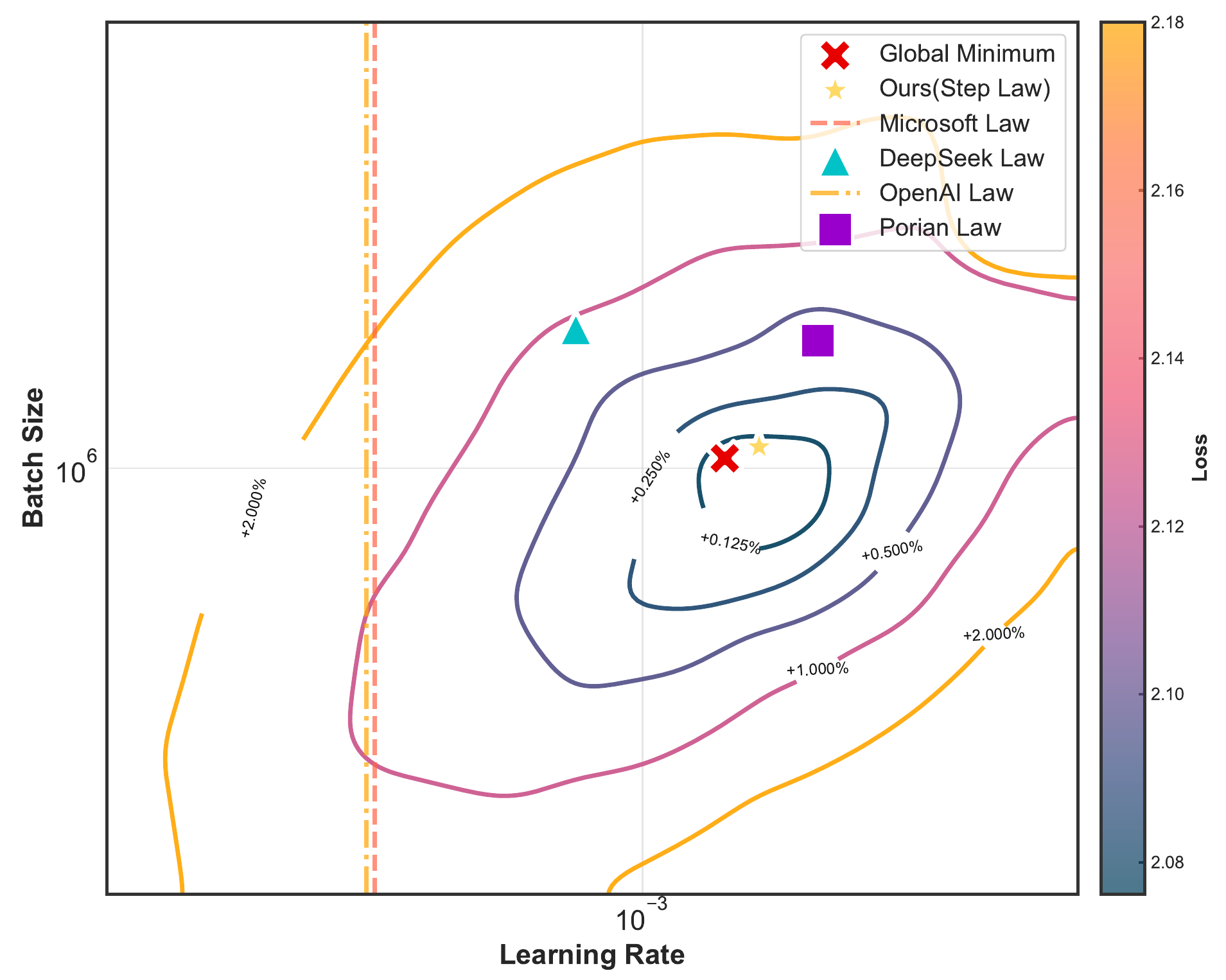
$\mu$-Transfer (Yang et al., 2022) supports width-direction LR transfer (including non-zero WD: original paper Appendix G.1.2; Power Lines). Limited experiments exist for BSZ, depth, and training-length directions; transfer to new recipes requires validation. Can be combined with hyperparameter power laws.
5.5 Search Procedure
Prioritize searching LR and BSZ, then check schedule and WD; stability hyperparameters such as $\epsilon$ and $\beta_2$ can be fixed after validation at baseline and representative scales. Use coordinate descent to iteratively narrow the range:
- Small model (~130M): grid search to identify core interval;
- Medium model (~500M): check power-law trend;
- Large model, local confirmation: LR can first be confirmed within the extrapolated value $\times/\div\,\sqrt{2}$; BSZ can first be confirmed within $[B/2,2B]$; expand if boundary checks warrant (§5.1, §5.3).
BSZ search dimensionality can be reduced using the transfer rules from §5.3. With LR already selected, adjusting WD to search for the optimal timescale $\tau = B/(\eta\lambda D)$ (Power Lines) reduces joint search cost; however, equal $\tau$ does not guarantee equivalent performance across different $(\eta, \lambda, B)$ triplets—LR stability and BSZ efficiency ranges still need checking.
5.6 Considerations When Comparing New Optimizers
Two key points from Fantastic Optimizers (Wen et al., 2025): each optimizer needs separate tuning with reported search budget—insufficiently tuned AdamW baselines exaggerate new optimizer gains; token efficiency improvement decreases with model size in their 8× Chinchilla experiments ($1.4\times$ at 0.1B down to $1.1\times$ at 1.2B), and is not equivalent to training-time speedup.
5.7 LR Schedule
Two commonly used schedules:
- Cosine: smooth decay to 0 or a small residual after short warmup. In multi-stage training, the minimum LR may differ across stages.
- WSD (Warmup-Stable-Decay): convenient for reusing the stable trajectory and annealing at a chosen budget. River Valley (Wen et al., 2024) explains the roles of the stable and decay phases under specific loss-geometry assumptions.
An annealing ratio of approximately 10%–20% can serve as an initial reference (Tissue et al., 2024); the target budget still requires validation. Wang et al., 2025 study cross-scale transfer of annealing strategies.
When comparing post-annealing delivery performance, annealing endpoints should be evaluated under comparable budgets. Fantastic Optimizers observed rank reversals during annealing; mid-stable rankings cannot directly substitute final rankings, except where validated proxy screening applies.
5.8 Finalization Steps
If the delivery pipeline includes the following steps, the corresponding Ladder stage should also execute them—or use a validated proxy—to keep fitting and delivery objectives aligned.
- Continued Training: after main training, switch data mix and decay LR (Nemotron-4, 2024; OLMo 2, 2025). When predicting final performance, this stage must be included (design in §8.1).
- Weight Averaging: averaging weights of checkpoints sharing the same initialization, including merging after independent fine-tuning (Model Soups) and sliding-window averaging along a single trajectory (LAWA; Sanyal et al., 2024). Model Merging (ByteDance Seed, 2025) found in 1.3B and 13B comparisons that PMA during the WSD stable phase can approach the downstream performance of the annealing endpoint; the merging window and starting point still require validation.
6. Loss Scaling Law and Downstream Task Fitting
Before fitting, three settings must be clarified (Porian et al., 2024):
- Compute accounting includes the output head, recorded separately from the fitting parameter count convention (§3.1)
- Warmup is set by scaling rule, avoiding disproportionate fractions at small budgets (§7.5)
- For objectives 2–4, each size is searched to the Fully-Tuned Frontier (§5.1); objective 1 runs by recipe
6.1 Functional Form
Chinchilla’s additive form implicitly assumes $\partial^2L/\partial N\partial D\equiv0$. Skaling (Videau et al., 2026) found a negative mixed partial derivative and introduced an outer exponent $k$:
\[L(N,D)=\left(\frac{A}{N^{\alpha}}+\frac{B}{D^{\beta}}\right)^{k}+E\]$k=1$ reduces to Chinchilla; fitted $k\approx0.31$–$0.45$. With only one additional parameter, the compute-optimal closed-form solution retains the same algebraic structure.
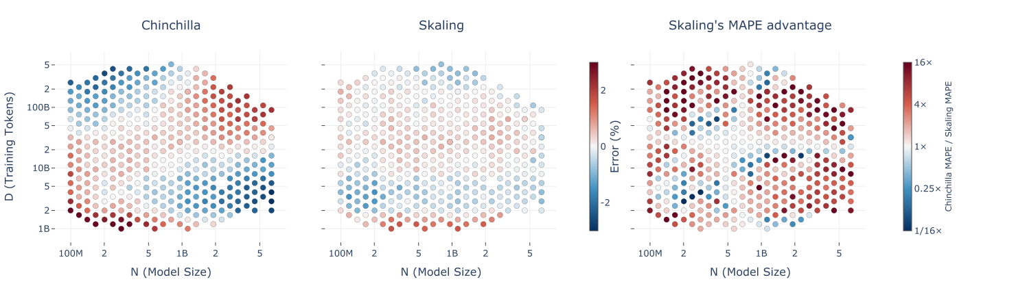
Farseer (Li et al., 2025) makes both the data-side coefficient and exponent dependent on $N$, totaling nine parameters. Skaling has six parameters and achieves the lowest interpolation and single-axis extrapolation error on both the Farseer and SK-Grid datasets (Skaling Table 1). Consider Skaling as the default candidate and compare against Chinchilla on your own data; refitting may change the compute-optimal ratio, which must be validated on the holdout.
At a fixed $D/N$, a one-dimensional approximation $L=G(M)/C^\gamma+E$ ($M=D/N$) can be used; cross-ratio modeling still requires $N$ and $D$.
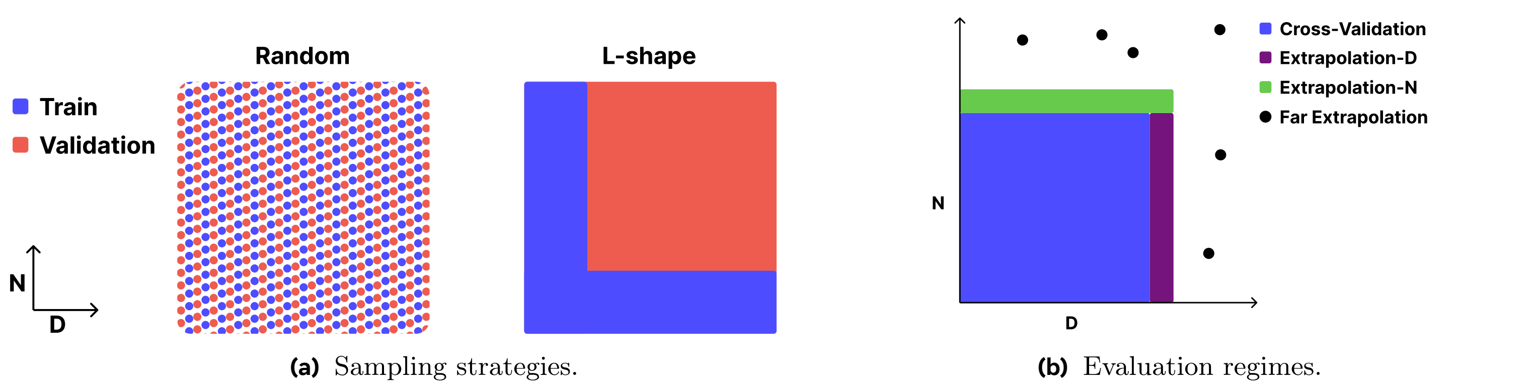
Layout should be jointly validated with functional form. In the two experimental setups from the Skaling paper, L-shape compute was reduced to roughly 1/5–1/10 of the full grid; the Chinchilla additive form showed noticeably increased error in these sparse experiments.
6.2 LR Annealing Scaling Law
Tissue et al., 2024 expresses loss as a function of step:
\[\hat L(s) = L_0 + A \cdot S_1(s)^{-\alpha} - C \cdot S_2(s)\]$S_1(s)=\sum_{i\leq s}\eta_i$ is the cumulative learning rate area, $S_2(s)$ is the cumulative annealing amount with a forgetting kernel. This formula takes the schedule as input, enabling fitting of the entire loss curve from multiple eval points along the same trajectory; it can also predict curves under different re-warmup LRs during continued training (original §4.7). Reusing coefficients across scales or data distributions still requires validation.
Personal experience: choosing a power-law kernel $K(\Delta) = (1+\Delta)^{-p}$ for the forgetting kernel typically outperforms the original paper’s single-exponential kernel.
6.3 Fitting Diagnostics and Failure Handling
After fitting, check:
- Residual structure: whether residuals show systematic variation with $N$, $D$, or training phase; whether conclusions depend on a few points or a specific functional form.
- Checkpoint correlation: multiple checkpoints from the same trajectory have serial correlation—independent information content cannot be judged by point count alone (Delphi bootstraps from IsoFLOP optimal points).
- Uncertainty decomposition: report seed variance, evaluation variance, and fitting uncertainty separately.
- Truncation and validation split: truncation rules should be predetermined or chosen on a development validation set; the holdout retains its acceptance role (§4.2).
- Failure handling: when errors are too large, specify experiments to be added and decisions that cannot yet be made. Explanations without evidence are recorded as “cause unknown.”
- Deliverables checklist: save recipe version, experiment log, fitting method, prediction intervals, and unresolved issues.
When decisions involve downstream capabilities, task metric predictions must also be validated; scaling regularities may differ across samples.
6.4 Downstream Prediction Methods
| Method | Core Idea | Representative Work | Limitations |
|---|---|---|---|
| Loss → Performance | First predict loss or perplexity, then map to downstream metrics | Gadre et al., 2024 (error rate power law on perplexity, equivalent to exponential on cross-entropy loss); Delphi (sigmoid) | Mapping depends on task and evaluation protocol |
| $(N,D)$ → Task Loss → Acc | Two-stage: first predict task-specific loss from $N,D$, then fit loss → accuracy | Bhagia et al., 2024 (OLMo Task Ladder) | Noise and prediction errors vary greatly across tasks |
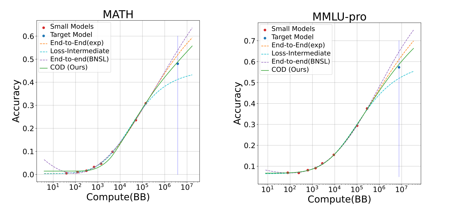
| End-to-End | Directly model task metrics vs. compute; can group by difficulty | COD (Xu et al., 2026, v4) (difficulty-feature clustering); GPT-4 Technical Report (HumanEval difficulty buckets) | Requires distinguishable evaluation signal; specific range depends on method and scoring protocol |
Delphi’s IsoFLOP + sigmoid mapping can serve as an initial approach. The strengths and weaknesses of different routes should be compared on the same tasks and protocol.
6.5 COD Framework Overview
The four-stage pipeline of COD (Xu et al., 2026, v4):
- Clustering: multiple small models sample each problem multiple times, using mean accuracy as the difficulty feature, then cluster by difficulty;
- Fitting: for each cluster fit $E[\mathrm{Acc}(C)] = g + (1-g) \cdot e^{-aC^{-b}-c}$;
- Extrapolation: filter reliable clusters, substitute target compute, and take sample-weighted average;
- Mapping: calibrate the mapping curve from the extrapolatable subset to the full evaluation set.
COD v4 achieves a mean absolute prediction error of 1.55 percentage points on a 70B model across 8 benchmarks (Table 1).
6.6 Applicability and Limitations
- When samples are too few, clustering metrics become unstable; under new architectures or data distributions, the stability of difficulty features and mappings must be validated.
- The main pre-training experiments use constant LR after warmup. Continued training experiments also involve data changes and annealing; small models must match the two-stage distribution and TPP (v4 Appendix D–E).
- v4 uses clusters derived from dense models to predict a 32B-active-parameter MoE target; mean and maximum absolute errors are 3.11 and 8.11 percentage points, providing limited cross-architecture evidence (§5.3.1, Table 2).
- CoT has empirical prediction results, but theory does not yet fully cover non-unique answers and reasoning paths (Appendix H).
7. Extrapolation Validation and Failure Handling
7.1 Holdout Validation
Set holdouts along the target extrapolation direction, with multiple extrapolation ratios arranged per budget. Delphi fits on 3e18–3e20 FLOPs, with holdouts up to 1e23 FLOPs; the first recipe’s loss was 2.5% above prediction at ~33× extrapolation, and the 333× run diverged.
After architecture or optimizer changes, first verify the transferability of old coefficients before deciding on local recalibration or full refitting (§3.4). Qwen3.8-Next, 2026 found that switching architecture + Muon shifted optimal LR and BSZ; after changes, the wide-plateau property (§5.1) can be used for local confirmation first, expanding the search if necessary.
The holdout error threshold must be determined in advance. Choshen et al., 2025 reports that the minimum relative difference driving modeling changes in the literature is about 4%, with random-restart fluctuations up to about 3.5%; Delphi’s 0.2%–0.5% is a specific experimental result and cannot serve as a universal acceptance threshold. Also report extrapolation confidence intervals.
7.2 Stability Stress Testing
Small-scale training cannot fully expose large-scale loss spikes and gradient anomalies. After architecture or optimizer changes, add stress tests: Qwen3.8-Next, 2026 uses medium-scale models with 2×/4× the predicted optimal LR to increase optimization pressure, comparing new and old recipes under the same pressure.
Short-duration stability at high LR and stability near the target training budget are different conditions. For critical candidates, record gradient norms, activation ranges, and routing statistics. Nemotron 3 Ultra (NVIDIA, 2026) §2.7 experienced two divergence events during late training—the first was related to output-layer gradient precision and stabilized after restoring FP32; the second had an unknown cause and was mitigated by early annealing.
Trajectories should be delivered together with stage configurations; investigation is triggered when the target training deviates.
7.3 Practical Efficiency and Deployment Constraints
Theoretical FLOPs improvements do not necessarily translate to proportional training-time improvements; actual training time should also be reported (Marin follow-up distinguishes theoretical and realized efficiency). Precision schemes require validation rather than assumed equivalence (Nemotron 3 Ultra). When inference deployment constraints exist, include inference cost in resource allocation.
7.4 Combination Validation
After individual modifications pass, the final combination should be validated; individual gains cannot simply be summed (Marin follow-up; OLMo 3, 2025 Appendix A.2.5). Key points:
- Data mix, training budget, and repetition degree should be checked jointly.
- Proxy experiment conclusions should state their transfer scope.
- Combination validation completed only at small scale cannot be stated as validated at target scale.
7.5 Common Pitfalls and Lessons
- Insufficient hyperparameter search: inadequate small-model search may bias hyperparameter extrapolation. Check search boundaries; timescale $\tau$ can organize joint search (§5.5).
- Inconsistent parameter count convention: mixing $N_{\text{body}}$ and total parameters, or substituting directly into $C=6ND$. Record the two conventions separately (§3.1).
- Excessive extrapolation range: loss curve scaling law (§6.2) shows systematic bias at large extrapolation ranges; supplement with additional experiment points.
- Early-training checkpoints: early points may cause systematic bias; truncation position should follow a predetermined rule or be chosen on a development set (§4.2). Truncation and warmup rules must be determined separately.
- Compute approximation: include the output head and attention computation per actual architecture (§3.2).
- Evaluation interval: fixed step intervals may give longer trajectories higher weight; sampling and weighting methods should be specified (§3.4, §6.3).
- Fitting formula: check whether the additive assumption fits your own data (§6.1).
8. Specific Scenarios
8.1 Multi-Stage Ladder
Different training stages have different data distributions, sequence lengths, and schedules; scaling law coefficients may change across stages (Qwen3, 2025; OLMo 3, 2025). For stages where configuration prediction or selection is needed, separate Ladders can be built:
- Pre-training Ladder: start from random initialization, fit $N$, $D$, LR, and BSZ;
- Mid-training Ladder: start from the corresponding pre-training checkpoint, fit additional token budget and LR schedule;
- Long-context Ladder: start from the corresponding mid-training checkpoint, search sequence length, RoPE configuration, and LR.
Scaling law coefficients should not be reused directly across stages; record both base capability changes and target capability increments.
8.2 MoE Ladder: Parameter Convention and Sparsity Axis
Each MoE experiment point must record: $N_{total}$ (total model parameters, including all experts), $N_{active}$ (parameters involved in computation per token, used to approximate FLOPs), total number of routed experts $E_{total}$ and routed experts activated per token $E_{active}$, sparsity ratio $S=E_{total}/E_{active}$ (shared experts recorded separately), router and load-balancing configuration.
Kimi K2, 2025 varies $E_{total}$ at fixed $N_{active}$ and FLOPs, fitting a sparsity scaling law: as sparsity increases from 8 to 48, the FLOPs needed to reach the same target loss decreases continuously, but communication and inference complexity increase. An MoE Ladder should include two types of experiments:
- Scale Ladder: fix sparsity ratio, vary $N_{active}$ and $D$;
- Sparsity Ladder: fix $N_{active}$, $D$, and active expert count, vary only $E_{total}$.
The fitting variables of the two experiment types must not be mixed.
8.3 Scaling Ladder Configuration References
Two relatively complete Ladder configurations from the published literature can serve as references, with different emphases:
8.3.1 Fantastic Optimizers Ladder (Dense, Hyperparameter-Search-Oriented)
Fantastic Optimizers (Wen et al., 2025) Tables 2–3. Llama 2 architecture; all four sizes fix 32 layers, MHA, seq_len 4096. The goal is fair optimizer comparison.
| Size | hidden_dim | inter_dim | heads | Data ratio |
|---|---|---|---|---|
| 130M | 512 | 2,048 | 8 | 1×–8× Chinchilla |
| 300M | 768 | 3,072 | 12 | Same |
| 520M | 1,024 | 4,096 | 16 | Same |
| 1.2B | 1,536 | 6,144 | 24 | Same |
Table 3 gives an AdamW search example (Peak LR 8e-3, WD 0.1, warmup 2000 steps, BSZ 128), which is the result for a specific size and ratio—different sizes have different configurations (e.g., 520M/1× uses WD 0.2, BSZ 256). Data is a mix of DCLM-baseline, StarCoder V2 Data, and ProofPile 2.
8.3.2 Delphi Ladder (End-to-End Scaling Law Oriented)
Delphi (Marin, 2026). Qwen 3 architecture, MLP ratio 4, seq_len 4096, dense decoder-only. The goal is to fit IsoFLOP scaling laws and extrapolate to 1e23 FLOPs (25B). Later extended to MoE (535B-A23B).
Shared settings: AdamH, WSD (10% warmup, 20% decay to 0), f32 parameters + bf16 compute, FSDP. Data: Nemotron-CC + StarCoderData + ProofPile 2.
Ladder structure: IsoFLOP sweep over 3e18–3e20 FLOPs; 7 optimal points used for fitting. Holdout 1e21–1e23 FLOPs (3×–333× extrapolation). Hyperparameters set by recipe rules, not manually searched per point.
8.3.3 Selection Guidance
- Need to search optimal hyperparameters and fit hyperparameter scaling laws → Fantastic Optimizers grid design
- Need end-to-end loss prediction extrapolated to large scale → Delphi IsoFLOP + recipe formula
- Both configurations are starting points; the model family and structural scaling rules should have proxy validity for the target large model (GQA, head_dim, width-depth configuration, etc.)
9. Build Checklist
9.1 Design Phase
- Define decision objectives (§1.4) and evaluation protocol (§2)
- Distinguish fixed quantities, scaling rules, and experimental independent variables (§3.4)
- Determine number of sizes and training-budget tiers, plus multiple holdout tiers (§4.2, §4.5, §7.1)
- Record $N_{\text{body}}$ and $C$ separately; tally FLOPs per actual architecture (§3.1, §3.2)
- For MoE, record total params, active params, and routing config; design scale and sparsity experiments separately (§8.2)
- If data mix is not yet determined, schedule mix experiments (§4.7)
- Design multi-stage training experiments as needed (§8.1)
- Under compute constraints, evaluate L-shape layouts (§6.1)
9.2 Configuration Phase
- Architecture attributes and scaling rules are consistent within the model family (§3.3); data, evaluation, and optimizer rules are consistent within the recipe (§3.4)
- Specify eval sampling and weighting rules, accounting for intra-trajectory correlation (§3.4, §6.3)
- Each metric has a distinguishable signal at Ladder scales (§2)
- If delivering a post-trained model, candidates need comparably conditioned SFT/RL acceptance (§2)
9.3 Search Phase
- Objectives 2–4: exhaustive search at small scale to the Fully-Tuned Frontier; objective 1: run by recipe (§5.1)
- Large-model LR: first confirm within $\times/\div\,\sqrt{2}$; BSZ: first confirm within $[B_{opt}/2,2B_{opt}]$; expand if necessary (§5.5, §5.3)
- Use $B_{opt}\propto D^{0.4}$ as BSZ prior, validate on own data (§5.3)
- When replicating a recipe, follow its WD; when studying cross-TPP relationships, check WD impact (§5.2)
9.4 Fitting Phase
- Verify FLOPs/parameter count convention and warmup rules (§6)
- Compare candidate functional forms (§6.1)
- For multi-epoch training, specify unique tokens and repetition count (§4.8)
- When using intermediate checkpoints, check the influence of early-training points; predetermine the truncation rule (§7.5)
- Check residual structure, correlation, and uncertainty decomposition; when errors are too large, record experiments to be supplemented (§6.3)
9.5 Validation Phase
- Predetermine holdout error threshold (§7.1)
- After architecture or optimizer changes, verify transferability and conduct stability stress tests (§7.1, §7.2)
- Downstream capability decisions require task metric prediction validation (§6.4)
- After individual modifications pass, validate the final combination (§7.4)
- Report both theoretical FLOPs and actual training time (§7.3)
- Save recipe version, experiment log, prediction intervals, and unresolved issues (§6.3)
10. References
Grouped by topic. Entries with section numbers have corresponding discussion in the main text.
Scaling Law Fundamentals and Functional Forms
- Scaling Laws for Neural Language Models — Kaplan et al., OpenAI, 2020. arXiv:2001.08361
Observed empirical power laws spanning 7 orders of magnitude in the tested range; for a given parameter count, width-depth ratio had little effect on loss. See §3.1, §3.2 - Training Compute-Optimal Large Language Models (Chinchilla) — Hoffmann et al., DeepMind, 2022. arXiv:2203.15556
IsoFLOP method and the result that model and data scale approximately proportionally; additive form $L=E+A/N^\alpha+B/D^\beta$. See §4.4 - Language models scale reliably with over-training and on downstream tasks — Gadre et al., 2024. arXiv:2403.08540
104 models validate that scaling laws remain reliable in the over-training regime; power-law exponents are similar across different $D/N$. See §4.4, §6.4 - Skaling: Chinchilla’s Exponents Meet Kaplan’s Coupling — Videau et al., FAIR at Meta, 2026. arXiv:2608.07222
Observed negative mixed partial derivative in the analyzed data, proposed the outer exponent $k$ and L-shape sampling, and validated their extrapolation performance. See §6.1 - Predictable Scale: Part II, Farseer — Li et al., StepFun & Fudan, NeurIPS 2025. arXiv:2506.10972
Nine-parameter form where data-side coefficient and exponent both explicitly depend on $N$; parameter count convention ablation. See §3.1, §6.1 - Scaling Law with Learning Rate Annealing — Tissue et al., 2024. arXiv:2408.11029
Expresses loss as a function of cumulative learning rate area and annealing amount, enabling full-curve fitting. See §6.2 - A Hitchhiker’s Guide to Scaling Law Estimation — Choshen et al., MIT/IBM, ICML 2025. arXiv:2410.11840
Intermediate checkpoints can be included in fitting but early unstable segments should be excluded; size count and extrapolation range discussed in main text. See §4.2, §7.1, §7.5 - Resolving Discrepancies in Compute-Optimal Scaling of Language Models — Porian et al., NeurIPS 2024. arXiv:2406.19146
Analyzes the impact of the output head, warmup, and hyperparameter tuning on compute-optimal exponent discrepancies. See §3.1, §6
Hyperparameter Scaling Laws
- DeepSeek LLM: Scaling Open-Source Language Models with Longtermism — DeepSeek, 2024. arXiv:2401.02954
Fits hyperparameter power laws by compute $C$; optimal resource allocation differs across the tested corpora; observes near-optimal hyperparameter intervals. See §4.6, §5.1, §5.4 - Predictable Scale: Part I — Optimal Hyperparameter Scaling Law in Large Language Model Pretraining (Step Law) — Li et al., StepFun, 2025. arXiv:2503.04715v3 $\eta_{opt}=c\,N^{-\alpha}D^{\beta}$, $B_{opt}=d\,D^{\gamma}$ validated on 3,700+ models. See §5.1, §5.4
- Power Lines: Scaling Laws for Weight Decay and Batch Size in LLM Pre-training — Bergsma et al., Cerebras, 2025. arXiv:2505.13738
Under their tested recipe, approximate relationships $B_{opt}\propto D^{0.4}$, $B_{crit}\propto D_{min}^{0.5}$ with weak $N$-dependence; timescale $\tau=B/(\eta\lambda D)$ can assist joint search given validated LR/BSZ rules and stability constraints. See §5.5, §5.3, §5.2 - Scaling Optimal LR Across Token Horizons — Bjorck et al., Microsoft, 2024. arXiv:2409.19913
At fixed model size, peak LR decays with training length. See §5.4 - Tensor Programs V: Tuning Large Neural Networks via Zero-Shot Hyperparameter Transfer ($\mu$-Transfer) — Yang et al., Microsoft, 2022. arXiv:2203.03466
Width-direction hyperparameter transfer under $\mu$P; limited experiments in other dimensions—transfer to new recipes requires validation. See §5.4 - Fantastic Pretraining Optimizers and Where to Find Them — Wen et al., Stanford, 2025. arXiv:2509.02046
Fair tuning benchmark across four sizes and 1×–8× Chinchilla; token efficiency gain varies with size and training budget; rank reversals may occur during annealing. See §5.6, §5.7, §8.3.1 - Weight Decay Improves Language Model Plasticity — Han et al., 2026. arXiv:2602.11137
In the tested setup, WD preferred by pre-training loss decreases with higher TPP; post-training plasticity may also benefit from stronger WD. See §5.2 - Small-Scale Experiments: Are We There Yet? — Lourie et al., NYU & Meta, 2026. arXiv:2608.11859
Small-model sensitivity to hyperparameters and the Fully-Tuned Frontier; sizes split into fitting, validation, and test segments—fitting choices determined on the validation segment. See §4.2, §5.1 - How to Allocate Your Tokens? Scaling Laws with Training Steps and Batch Size — Schaipp, Inria, 2026. arXiv:2607.01487
Defines near-optimal batch interval by loss-equivalent compute loss; measured interval width is approximately fourfold. See §5.3
Data and Training Budget
- Scaling Data-Constrained Language Models — Muennighoff et al., 2023. arXiv:2305.16264
Equivalent token quantity formula for repeated data and marginal return decay curve. See §4.8 - To Repeat or Not To Repeat: Insights from Scaling LLM under Token-Crisis — Xue et al., 2023. arXiv:2305.13230
Controlled experiments analyzing the impact of parameter count, data quantity, and quality on repetition overfitting; dropout effectiveness and rate need scale-specific validation. See §4.8 - Prescriptive Scaling Laws for Data Constrained Training — Lovelace et al., 2026. arXiv:2605.01640
Models overfitting jointly driven by parameter count, unique tokens, and repetition count in the tested range. See §4.8 - Larger Datasets Can Be Repeated More: A Theoretical Analysis of Multi-Epoch Scaling in Linear Regression — Yan et al., 2025. arXiv:2511.13421
Under specific linear-regression assumptions, analyzes the relationship between repetition count and dataset sample size, with LLM experiments. See §4.8
LR Schedule and Training Finalization
- Understanding Warmup-Stable-Decay Learning Rates: A River Valley Loss Landscape Perspective — Wen et al., 2024. arXiv:2410.05192
Under specific loss geometry and optimization dynamics assumptions, explains the roles of the WSD stable and decay phases. See §5.7 - Scaling and Transferability of Annealing Strategies in Large Language Model Training — Wang et al., 2025. arXiv:2512.13705
Scaling and cross-scale transfer of annealing strategies. See §5.7 - Model Merging in Pre-training of Large Language Models — ByteDance Seed, 2025. arXiv:2505.12082
Studies checkpoint merging during pre-training; in specific comparisons, stable-phase PMA approaches annealing-endpoint performance. See §5.8 - Model Soups: Averaging Weights of Multiple Fine-tuned Models — Wortsman et al., 2022. arXiv:2203.05482
Weight averaging of models independently fine-tuned from a shared pre-trained starting point. See §5.8 - Stop Wasting My Time! Saving Days of ImageNet and BERT Training with Latest Weight Averaging (LAWA) — Kaddour, 2022. arXiv:2209.14981
Sliding-window weight averaging along a single trajectory. See §5.8 - Early Weight Averaging meets High Learning Rates for LLM Pre-training — Sanyal et al., COLM 2024. arXiv:2306.03241
Early weight averaging under high learning rates. See §5.8
Downstream Task Prediction
- Unveiling Downstream Performance Scaling of LLMs: A Clustering-Based Perspective (COD) — Xu et al., ICLR 2026, v4 (2026-03-09). arXiv:2502.17262v4 Clusters by difficulty features, filters predictable clusters, and maps to the full set; includes dense and MoE target prediction and continued training experiments. See §6.4–§6.6
- GPT-4 Technical Report — OpenAI, 2023. arXiv:2303.08774
Buckets HumanEval by difficulty based on small-model performance and fits extrapolation on subsets. See §6.4 - Establishing Task Scaling Laws via Compute-Efficient Model Ladders (OLMo Task Ladder) — Bhagia et al., Allen Institute, 2024. arXiv:2412.04403
Two-stage downstream prediction: first fit task-specific loss from $N,D$, then fit loss → accuracy; significant noise variation across tasks. See §6.4
Model Technical Reports and Ladder Instances
- Delphi: An Open Scaling Suite from 3e18 to 1e23 FLOPs — Marin Team, 2026. openathena.ai/blog/delphi
IsoFLOP fitting + recipe-formula-driven hyperparameters; multi-tier holdout extrapolation. See §1.2, §7.1, §8.3.2 - Nemotron-4 15B Technical Report — NVIDIA, 2024. arXiv:2402.16819
Batch size ramp-up strategy; continued training at end of training. See §5.8 - OLMo: Accelerating the Science of Language Models — Groeneveld et al., Allen Institute, 2024. arXiv:2402.00838
Fully open training data, code, and intermediate checkpoints. See §4.3 - OLMo 2: The Next Generation of Fully Open Language Models — OLMo Team, Allen Institute, 2025. arXiv:2501.00656
Two-stage training; Micro-annealing for low-cost data source validation; model souping. See §4.6, §5.8 - OLMo 3 — Allen Institute, 2025. arXiv:2512.13961
Multi-stage training configuration and integrated validation; Dirichlet data-mix process; effective-scale calibration of evaluation metrics. See §8.1, §4.7, §2 - Qwen3 Technical Report — Qwen Team, 2025. arXiv:2505.09388
Stage-wise prediction of LR and batch size; data mix along instance attribute dimensions. See §8.1, §4.7 - On the Design of Qwen3.8-Next Architecture — Qwen Team, 2026. arXiv:2608.30320
Hyperparameter shifts after architecture and optimizer changes; stability stress testing methodology. See §7.1, §7.2 - Kimi K2: Open Agentic Intelligence — Moonshot AI, 2025. arXiv:2507.20534
Studies routed expert sparsity ratio and compute efficiency at fixed active scale. See §8.2, §5.2 - Nemotron 3 Ultra Technical Report — NVIDIA, 2026. PDF
High-precision branch comparisons during training, demonstrating that precision schemes require validation. See §7.3 - Marin: MoE and Training Efficiency Follow-Up — Marin Team, 2026. openathena.ai/blog/pretraining-speedup
Distinguishes theoretical and realized efficiency; multi-scale recipe comparison, pre-registered predictions, and combination experiment design. See §7.3, §7.4, §8.3.2
Further Reading
The following works are related to Ladder design but not expanded upon in the main text:
- Chinchilla Scaling: A Replication Attempt — Besiroglu et al., Epoch AI, 2024. arXiv:2404.10102
- (Mis)Fitting: A Survey of Scaling Laws — Li et al., 2025. arXiv:2502.18969
- Beyond Chinchilla-Optimal: Accounting for Inference in Language Model Scaling Laws — Sardana et al., 2024. arXiv:2401.00448
- Critical Batch Size Revisited: A Simple Empirical Approach to Large-Batch Language Model Training — Merrill et al., 2025. arXiv:2505.23971
- An Empirical Model of Large-Batch Training — McCandlish et al., 2018. arXiv:1812.06162
- GQA: Training Generalized Multi-Query Transformer Models from Multi-Head Checkpoints — Ainslie et al., Google, 2023. arXiv:2305.13245
- Cost-Optimal Grouped-Query Attention for Long-Context Modeling — Chen et al., 2025. arXiv:2503.09579
- Nemotron-4 340B Technical Report — NVIDIA, 2024. arXiv:2406.11704